Pitfalls using MAPE as forecast accuracy metric
Introduction
Despite being a very popular metric for measuring forecast accuracy in forecasting, MAPE certainly has its strengths and limitations that anyone using it should take into consideration. This deep review of the efficacy of MAPE for measuring forecast accuracy in any kind of forecasting task like heat demand, solar- or wind power and inspect the metric’s behavior in different scenarios. For scenarios where MAPE is not suitable, alternative metrics are discussed.
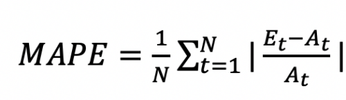
The equation shows how the MAPE is calculated. E_t is the extimated/predicted value at specific time and A_t is the Actual or Observed/Measured value at specific time. N is the number of timesteps (or length of dataset) to derive MAPE for.
MAPE (Mean Absolute Percentage Error)
Strengths
- Easy to Interpret: MAPE is easy to understand. For example, if MAPE for monthly demand forecasts of a product is 10% over the last 12 months, it means that forecasts were wrong by 10% on average over this time period.
- Scale Independent: MAPE is suitable for comparisons across different data sets as it is scale independent.
Limitations
-
Bias for Very Low Values and Outliers:
- MAPE can get significantly inflated due to low values or outliers.
- Example: A drop in observed values to 20 units can result in an absolute percentage error (APE) of 6000%, affecting the overall MAPE.
-
Intermittent Values:
- MAPE becomes infinite or undefined for data with zero values periods, making it unsuitable for assessing forecast accuracy in such cases.
-
Asymmetry:
- MAPE can appear asymmetric because over-predictions can result in a higher MAPE compared to under-predictions.
-
Directionless:
- MAPE does not reflect the direction of errors (over-predictions vs. under-predictions), which can be crucial in supply chain demand planning.
Alternatives to MAPE
RMSE (Root Mean Squared Error)
- The root mean square error (RMSE) measures the average difference between a statistical model’s predicted values and the actual values.
- Mathematically, it is the standard deviation of the residuals. Residuals represent the distance between the regression line and the data points.
WAPE (Weighted Absolute Percentage Error)
- Defined as the sum of absolute errors divided by the sum of actual values.
- Like MAPE, it is scale-free but does not get inflated by small values.
MdAPE (Median Absolute Percentage Error)
- More resistant to outliers compared to MAPE.
MASE (Mean Absolute Scaled Error)
- Scales forecast errors by the in-sample, one-step-ahead MAE of the Naïve method.
- Suitable for intermittent values but less intuitive to interpret.
sMAE (Scaled MAE)
- Uses the in-sample actual values mean as the scaling factor.
- More intuitive than MASE but problematic for non-stationary data.
Practical Implications
- Blindly optimizing for MAPE can result in sub-optimal forecasts.
- WAPE can be a better alternative in scenarios where MAPE’s limitations are pronounced.
Summary
- Intuitive and Suitable for Comparisons: MAPE is easy to understand and compare.
- Handling Trade-offs: For trade-offs between over-prediction and under-prediction, MAPE can be split into components.
- Skewed Distribution: MAPE is not suitable for data with periods of low values or intermittent values.
- Asymmetry in Predictions: MAPE is unbounded for over-predictions and can lead to conservative forecasts.
- Alternative Metrics: WAPE is a scale-free metric that addresses many concerns of MAPE while retaining similar strengths.
References
- Armstrong, J. Scott, and Fred Collopy. 1992. “Error Measures for Generalizing about Forecasting Methods: Empirical Comparisons.” International Journal of Forecasting 8(1). doi: 10.1016/0169-2070(92)90008-W.
- Goodwin, Paul, and Richard Lawton. 1999. “On the Asymmetry of the Symmetric MAPE.” International Journal of Forecasting 15(4):405–8. doi: 10.1016/S0169-2070(99)00007-2.